43 add data labels to scatter plot excel 2007

Labeling X-Y Scatter Plots (Microsoft Excel) - ExcelTips (ribbon) Just enter "Age" (including the quotation marks) for the Custom format for the cell. Then format the chart to display the label for X or Y value. When you do this, the X-axis values of the chart will probably all changed to whatever the format name is (i.e., Age). Plot a graph from list, dataframe in Python | EasyTweaks.com Note: you can create plots also from Excel files. Use the pd.read_excel() method to import your Excel data into a DataFrame and then render your graph as shown in the last section of this post. Additional Learning. How to create a Scatter plot with Python?

How to Insert Axis Labels In An Excel Chart | Excelchat We will again click on the chart to turn on the Chart Design tab. We will go to Chart Design and select Add Chart Element. Figure 6 - Insert axis labels in Excel. In the drop-down menu, we will click on Axis Titles, and subsequently, select Primary vertical. Figure 7 - Edit vertical axis labels in Excel. Now, we can enter the name we want ...

Add data labels to scatter plot excel 2007

Create a chart from start to finish - support.microsoft.com You can create a chart for your data in Excel for the web. Depending on the data you have, you can create a column, line, pie, bar, area, scatter, or radar chart. Click anywhere in the data for which you want to create a chart. To plot specific data into a chart, you can also select the data. Text Labels on a Horizontal Bar Chart in Excel - Peltier Tech 21.12.2010 · In Excel 2003 the chart has a Ratings labels at the top of the chart, because it has secondary horizontal axis. Excel 2007 has no Ratings labels or secondary horizontal axis, so we have to add the axis by hand. On the Excel 2007 Chart Tools > Layout tab, click Axes, then Secondary Horizontal Axis, then Show Left to Right Axis. Labeling X-Y Scatter Plots (Microsoft Excel) Just enter "Age" (including the quotation marks) for the Custom format for the cell. Then format the chart to display the label for X or Y value. When you do this, the X-axis values of the chart will probably all changed to whatever the format name is (i.e., Age).

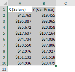
Add data labels to scatter plot excel 2007. Present your data in a bubble chart - support.microsoft.com A bubble chart is a variation of a scatter chart in which the data points are replaced with bubbles, and an additional dimension of the data is represented in the size of the bubbles. Just like a scatter chart, a bubble chart does not use a category axis — both horizontal and vertical axes are value axes. In addition to the x values and y values that are plotted in a scatter chart, … Improve your X Y Scatter Chart with custom data labels Select the x y scatter chart. Press Alt+F8 to view a list of macros available. Select "AddDataLabels". Press with left mouse button on "Run" button. Select the custom data labels you want to assign to your chart. Make sure you select as many cells as there are data points in your chart. Press with left mouse button on OK button. Back to top peltiertech.com › text-labels-on-horizontal-axis-in-eText Labels on a Horizontal Bar Chart in Excel - Peltier Tech Dec 21, 2010 · In Excel 2003 the chart has a Ratings labels at the top of the chart, because it has secondary horizontal axis. Excel 2007 has no Ratings labels or secondary horizontal axis, so we have to add the axis by hand. On the Excel 2007 Chart Tools > Layout tab, click Axes, then Secondary Horizontal Axis, then Show Left to Right Axis. Add Custom Labels to x-y Scatter plot in Excel Step 1: Select the Data, INSERT -> Recommended Charts -> Scatter chart (3 rd chart will be scatter chart) Let the plotted scatter chart be. Step 2: Click the + symbol and add data labels by clicking it as shown below. Step 3: Now we need to add the flavor names to the label. Now right click on the label and click format data labels.

› charts › stem-and-leaf-templateHow to Create a Stem-and-Leaf Plot in Excel - Automate Excel To do that, right-click on any dot representing Series “Series 1” and choose “Add Data Labels.” Step #11: Customize data labels. Once there, get rid of the default labels and add the values from column Leaf (Column D) instead. Right-click on any data label and select “Format Data Labels.” When the task pane appears, follow a few ... excel - How to label scatterplot points by name? - Stack Overflow 14.04.2016 · I am currently using Excel 2013. This is what you want to do in a scatter plot: right click on your data point. select "Format Data Labels" (note you may have to add data labels first) put a check mark in "Values from Cells" click on "select range" and select your range of labels you want on the points; UPDATE: Colouring Individual Labels › excel-charting-and-pivotsScatter Plot not showing all data points - Excel Help Forum Sep 17, 2019 · I created a scatter plot based on a table with 25 data coordinates but (1) only 16 coordinates are showing in the scatter plot and (2) some of the labels on the scatter plot aren't showing. Does anyone know how I can fix this? Images are below. Here's some other information that might be useful: - I'm using Excel for Mac 2019 (standalone version). support.microsoft.com › en-us › officeCreate a chart from start to finish - support.microsoft.com You can create a chart for your data in Excel for the web. Depending on the data you have, you can create a column, line, pie, bar, area, scatter, or radar chart. Click anywhere in the data for which you want to create a chart. To plot specific data into a chart, you can also select the data.

Excel 2007 : Labels for Data Points on a Scatter Chart Re: Labels for Data Points on a Scatter Chart The addin is not required by anybody receiving your workbook. The addin will link the data label to a cell. If the cell changes the data label will change. New data points will not automatically be linked to new cells. That would require the use of the addin, in order to avoid do it manually. How to Add Labels to Scatterplot Points in Excel - Statology Step 3: Add Labels to Points. Next, click anywhere on the chart until a green plus (+) sign appears in the top right corner. Then click Data Labels, then click More Options…. In the Format Data Labels window that appears on the right of the screen, uncheck the box next to Y Value and check the box next to Value From Cells. How do you define x, y values and labels for a scatter chart in Excel 2007 By default, the single series name appears in the chart title and in the legend. Your third post included steps for creating an XY chart with three data series, each with a single data point, so that the "label" is used as the name of the data series. The data series name then appears in the chart legend. How to Create a Panel Chart in Excel – Automate Excel Step #1: Add the separators. Before you can create a panel chart, you need to organize your data the right way. First, to the right of your actual data (column E), set up a helper column called “Separator.” The purpose of this column is to split the data into two alternating categories—expressed with the values of 1 and 2—to lay the groundwork for the future pivot …

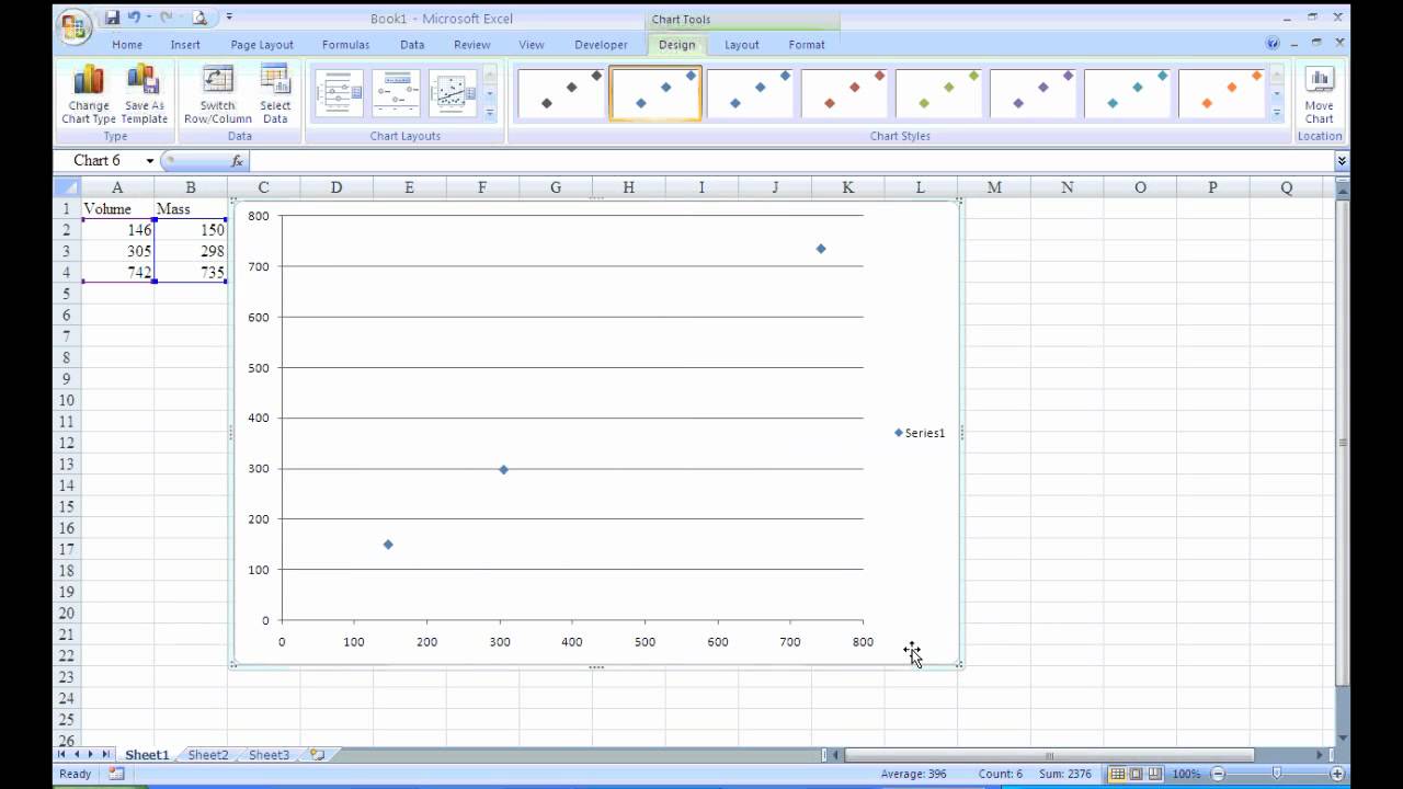
Excel Data Entry, Scatter Plots, and Export - YouTube

› dynamically-labelDynamically Label Excel Chart Series Lines • My Online ... Sep 26, 2017 · Great question. Pivot Charts won’t allow you to plot the dummy data for the label values in the chart as it wouldn’t be part of the source data, so the options are: 1. create a regular chart from your PivotTable and add the dummy data columns for the labels outside of the PivotTable. Not ideal if you’re using Slicers.

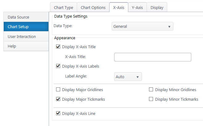
Chart Plus – Bamboo Solutions

How to Quickly Add Data to an Excel Scatter Chart - EngineerExcel The first method is via the Select Data Source window, similar to the last section. Right-click the chart and choose Select Data. Click Add above the bottom-left window to add a new series. In the Edit Series window, click in the first box, then click the header for column D. This time, Excel won't know the X values automatically.

How Do I Use Scatter Plots in Excel? (with Pictures) | eHow

How to Add Data Labels to an Excel 2010 Chart - dummies Use the following steps to add data labels to series in a chart: Click anywhere on the chart that you want to modify. On the Chart Tools Layout tab, click the Data Labels button in the Labels group. None: The default choice; it means you don't want to display data labels. Center to position the data labels in the middle of each data point.

Excel: labels on a scatter chart, read from array - Stack Overflow

peltiertech.com › prevent-overlapping-data-labelsPrevent Overlapping Data Labels in Excel Charts - Peltier Tech May 24, 2021 · Overlapping Data Labels. Data labels are terribly tedious to apply to slope charts, since these labels have to be positioned to the left of the first point and to the right of the last point of each series. This means the labels have to be tediously selected one by one, even to apply “standard” alignments.

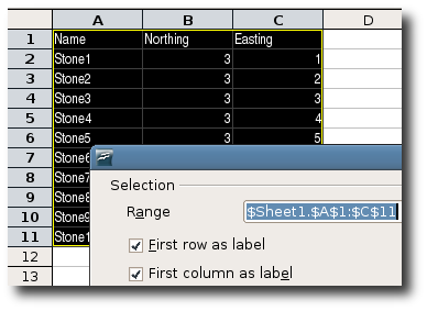
How to Label Excel and OpenOffice.org XY Scatter Plots

Add data labels to your Excel bubble charts | TechRepublic Right-click the data series and select Add Data Labels. Right-click one of the labels and select Format Data Labels. Select Y Value and Center. Move any labels that overlap. Select the data labels ...

30 Label Scatter Plot Excel - Labels Design Ideas 2020

Prevent Overlapping Data Labels in Excel Charts - Peltier Tech 24.05.2021 · Overlapping Data Labels. Data labels are terribly tedious to apply to slope charts, since these labels have to be positioned to the left of the first point and to the right of the last point of each series. This means the labels have to be tediously selected one by one, even to apply “standard” alignments.

graph - X-Y scatter plots in excel - Stack Overflow

Add labels to data points in an Excel XY chart with free Excel add-on ... Next, open your Excel sheet and click on the new "XY Chart Labels" menu that appears (above the ribbon). Next, click on "Add Labels" in order to determine the range to use for your labels. In the dialog that appears, select the range where your labels will be coming from (as illustrated below in this example) You will get the result below:

How to Make a Scatter Plot in Excel to Present Your Data

How to Create a Stem-and-Leaf Plot in Excel - Automate Excel Step #10: Add data labels. As you inch toward the finish line, let’s add the leaves to the chart. To do that, right-click on any dot representing Series “Series 1” and choose “Add Data Labels.” Step #11: Customize data labels. Once there, get rid of the default labels and add the values from column Leaf (Column D) instead.

How to Create a Scatter Plot in Excel

How to label scatterplot points by name? - Stack Overflow 13 Apr 2016 — right click on your data point · select "Format Data Labels" (note you may have to add data labels first) · put a check mark in "Values from Cells ...5 answers · Top answer: Well I did not think this was possible until I went and checked. In some previous version of ...Adding Names to Scatter Plot Points Without Modifying X ...12 Jul 2016Excel 2007, How to avoid scatter chart data points overlap3 Feb 2018Add hover labels to a scatter chart that has it's data range ...15 Jul 2012Adding webpage link to each data point or data label on an ...22 May 2017More results from stackoverflow.com

How to Create a Scatter Plot in Excel

How to find, highlight and label a data point in Excel scatter plot Add the data point label To let your users know which exactly data point is highlighted in your scatter chart, you can add a label to it. Here's how: Click on the highlighted data point to select it. Click the Chart Elements button. Select the Data Labels box and choose where to position the label.

Improve your X Y Scatter Chart with custom data labels

How do I set labels for each point of a scatter chart? Click one of the data points on the chart. Chart Tools. Layout contextual tab. Labels group. Click on the drop down arrow to the right of:- Data Labels Make your choice. If my comments have helped please vote as helpful. Thanks. Report abuse Was this reply helpful? Yes No

How to Change Labels for a Chart Axis in Excel 2007

Add Data Labels To Excel Scatter Plot - how-use-excel.com Add or remove data labels in a chart. Excel Details: On the Design tab, in the Chart Layouts group, click Add Chart Element, choose Data Labels, and then click None.Click a data label one time to select all data labels in a data series or two times to select just one data label that you want to delete, and then press DELETE. Right-click a data label, and then click Delete. excel scatter plot ...

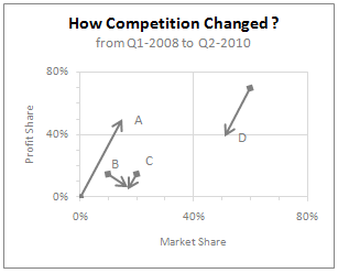
Analyzing & Visualizing Competition - Free Excel Business Chart Template | Chandoo.org - Learn ...

AutoFilter Changes Data Labels In 2007 Chart - Excel General - OzGrid ... I have a scatter chart and have applied data labels using the VBA macro supplied with Excel 2007. They pick up the cells in column A. But I now want to use Autofilter to show different ranges in the chart. ... He's used the macro supplied by MS to add data labels to a scatter chart and is having the same problem when filtering. I have added the ...

Scatter Plot in Excel - Easy Excel Tutorial

Apply Custom Data Labels to Charted Points - Peltier Tech First, add labels to your series, then press Ctrl+1 (numeral one) to open the Format Data Labels task pane. I've shown the task pane below floating next to the chart, but it's usually docked off to the right edge of the Excel window. Click on the new checkbox for Values From Cells, and a small dialog pops up that allows you to select a ...

How to have a color-specified scatter plot in excel? - Super User

Adding Data Labels to a Chart Using VBA Loops - Wise Owl To do this, add the following line to your code: 'make sure data labels are turned on. FilmDataSeries.HasDataLabels = True. This simple bit of code uses the variable we set earlier to turn on the data labels for the chart. Without this line, when we try to set the text of the first data label our code would fall over.

X-Y scatter plot in Excel 2007 - YouTube

Dynamically Label Excel Chart Series Lines - My Online Training … 26.09.2017 · Great question. Pivot Charts won’t allow you to plot the dummy data for the label values in the chart as it wouldn’t be part of the source data, so the options are: 1. create a regular chart from your PivotTable and add the dummy data columns for the labels outside of the PivotTable. Not ideal if you’re using Slicers.

Share :